Great Scott! Timing Attack Demo for the Everyday Webdev

One of the more insidious ways your web application’s data can be comprised is through a timing attack. The time it takes your app to serve a request can reveal more information than you might think. While certain ingredients need to be present for a successful timing attack, the surface area is large and we can’t depend on a library to protect us against all cases.

After you understand the ins and outs of a timing attack, you might be surprised at what you find auditing your own web application. What follows below is a complete walk through extracting secret data from a vulnerable demo application.

The scripts are written in Ruby, and while we love it if that’s not your language don’t worry!  Written explanations are provided for each code snippet.

The demo app and all code in this timing attack walkthrough can be found here on the Simple Thread Github page.

Demo App Overview

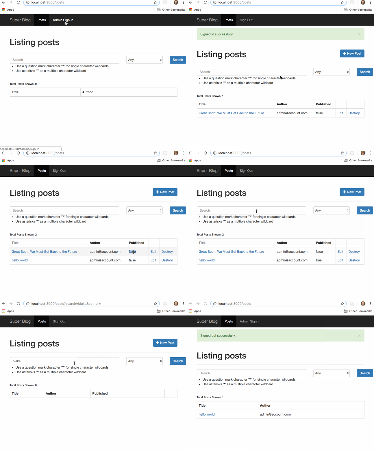
Before we get to the good stuff, here is the vulnerable demo app, which we will call Great Scott, a standard CRUD blog. Any user that visits the site can search posts by title (case insensitive) or author. When you log in as an admin you have the ability to create and publish posts. Only the admin can see unpublished blog posts.

The timing attack vector will be abusing the search feature to grab the title of unpublished blog posts by measuring the time it takes for the server to respond.

Minimal Proof

As the attacker, the easiest place to start is creating a minimal test to see if a timing attack is possible. The goal of a minimal test isn’t to fully extract the secret title. We’re going to pass two search queries and measure the results. One will match a piece of the title and the other won’t.

Let’s set up our lab environment to remove as many variables as possible for the timing attack. We’ll be running our exploit scripts and app server on the same box so jitter caused by going over the open internet won’t be an issue. Also we’ll kill any resource hungry processes. Finally we want only one blog post to exist in our application and it should be unpublished. The rest of the guide assumes the title of this post is “Great Scott! We Must Get Back to the Future”

Before running any scripts yourself make sure you only have a single unpublished post! Additional posts adds “noise” and we’ll discuss overcoming that later. You can run the setup commands listed in the README to reset the database and create this single unpublished post.

To start we’ll build a simple method to wrap the search route. For all intents and purposes this is basically curl.

Next we want to measure how long it takes for the server to respond. We’ll wrap our get method above with a benchmark to measure the time it takes for the server to respond in milliseconds:

Now we’re ready to actually build our test case. We’ll test two search terms: ‘scott,’ and ‘blake’. ‘scott’ is in the unpublished post’s title while ‘blake’ is not. We’ll run 100 trials each by passing the term into the previously defined benchmark_get method. The results variable contains the search term and an array of runtimes.

See full script here

Finally let’s do some number crunching on the results.

Term: scott
Trials: 100
Min: 87.3
Max: 135.3
Mean: 95.7
Standard Deviation: 6.7

Term: blake
Trials: 100
Min: 75.6
Max: 161.1
Mean: 84.7
Standard Deviation: 11.5

( Results will vary )

The first thing to note is that there is a noticeable gap between the averages. “Scott” took ever slightly longer to run. Approximately 10ms longer to run then “blake”. That’s seems like a positive result but how can we be sure? Request times can vary after all, just take a look at the minimum and maximum result for each term. Maybe if we ran this script again “blake” might come back with a higher average? Maybe this was just dumb luck?

Rephrasing those questions in a more scientific way: how do we know the results are statistically significant? That’s where computing a confidence interval comes in.  A confidence interval gives us a range that likely includes the true mean. You can read more about how this value is computed here.

Term: scott
Confidence Interval 95%: [94.3, 96.9]
Confidence Interval 99%: [93.9, 97.4]

Term: blake
Confidence Interval 95%: [82.4, 87.0]
Confidence Interval 99%: [81.6, 87.7]

For “scott” we are 99% sure that our confidence interval of 93.9ms to 97.4ms contains the true mean.  For “blake” we are 99% sure that our confidence interval of 81.6ms to 87.7ms contains the true mean. Since there is a gap between the low end of scott’s range and the high end of blake’s range we can draw a reasonable conclusion. Yes there indeed is a measurable difference when a search query contains text from an unpublished post title.

Extracting Title Length

Now that we’ve established that there’s a measurable difference, how do we extract the full title? We could just start by feeding single characters into a query. Doing so would allow us to confirm there’s say one or more ‘A’ characters somewhere in the title but we wouldn’t know the location. Also how would we know when we’ve extracted the full title and can stop? Wouldn’t it be nice if we could determine the length of the secret title first?

Take a closer look at those search options. “Use a ‘?’ for single character wildcards” Let’s put it to good use.

See full script here

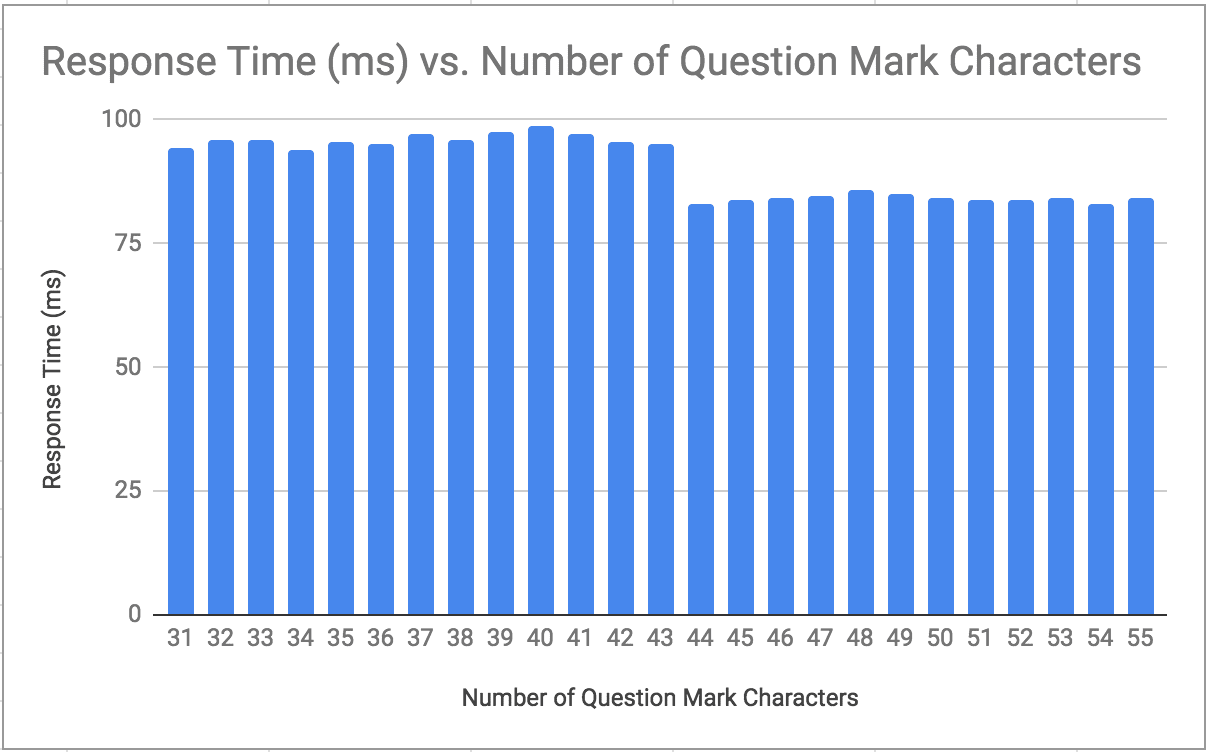
We feed in a series of queries with an increasing number of question marks. e.g. “?”, “??”, “???”

Let’s chart the mean:

Our title is “Great Scott! We Must Get Back to the Future” which is 43 characters. Notice the dip in results between between passing queries with 43 and 44 question marks? We’ve determined the character length of the secret blog post from the attacker’s perspective.

There’s an additional benefit to extracting the title length first. When we move out of the lab environment and have multiple posts in the system, then published posts will add processing time and thus help “cover up” unpublished posts. As the attacker, being able to filter by title length means an unpublished post with a unique character count is ripe for the picking.

Coup De Grâce

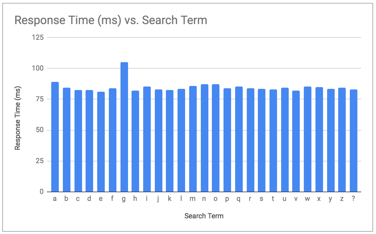
To get the first letter of our hidden post title we can iterate from ‘a’ to ‘z’ with 42 wildmark characters (question marks). That makes 43 characters total.

Let’s chart the mean result for each letter:

Notice the “g” stands out? We’ve extracted the first letter of the post. Before we go adding a loop and calling it a day we should consider two additional things.

First is that we are only querying for alphabetic letters. What happens when our script hits the “!” character? We need a way to differentiate when the character we’re scanning for doesn’t exist in our list. Ultimately we can skip these characters and come back after extracting the alphabetic characters with a list of educated guess characters.

If the leading result doesn’t stand out then we can conclude that the character doesn’t exist in our list. An easy way to check this is to calculate the difference (delta) between the leading character’s mean and mean of all results. In our algorithm we’ll set a delta threshold value that determines whether we accept the winning result or leave the character as a wildcard “?” and continue on.

The second issue is the huge number of requests this is going to take. So far we’ve been using 100 trials/requests per a query term. The minimal proof script resulted in 200 requests total. Extracting the title length took 6,000 requests. If you’ve been following along with the repo you will have noticed a significant jump in time to run those two scripts. Now if we stay our current course it’s going to take us 111,800 requests. (43 characters in the title * 26 characters * 100 trials )

Can we dial back the number of requests we’re running per character? Well, as we decrease the number of requests the outlying results are going to have a greater impact. Take a look back at the results for the initial proof of concept test. “blake” actually had the higher maximum result even though it’s average was significantly less than “scott”. Over 100 trials this result was “smoothed” over by a series of typical results into a mean that was less than “scott”. As we decrease the number of trials we’re going to get less of this smoothing effect and our mean will include more noise.

One way of working with less data is checking whether the data is tightly grouped or contains big outliers. If the data contains huge outliers we can throw out the results and try again. We can use standard deviation for this but that value will scale as the run time changes and we would need to keep constantly adjusting our threshold. We can normalize this value as a percentage by dividing the standard deviation against the mean. This is called Coefficient of Variation.

By doing this check we can reduce the number of trials per character to 10. Sometimes the winning character isn’t going to be clear. In those cases we’ll have to throw out the results and try again. Even so, this is going to come out to considerably less requests than sticking with 100 trials each for our upcoming timing attack.

Let’s put it all together in the final code.

See final code here

Note that depending on your environment you may need to tweak the constants at the top of the script.  Here’s a snippet of output:

Trial 1 of 10
Trial 2 of 10
Trial 3 of 10
Trial 4 of 10
Trial 5 of 10
Trial 6 of 10
Trial 7 of 10
Trial 8 of 10
Trial 9 of 10
Trial 10 of 10
Exporting results to csv...
tmp/1548447356.csv
Delta: 16.7114306526752
Coefficient Variation: 9.705968406065965
Current Secret: great sc*??????????????????????????????????

Additional Optimizations

There’s plenty more you could do to optimize this further.

• The attacking script could be optimized by short circuiting after one character’s result has an anomaly.
• The attacker could use letter frequencies to start with more likely characters instead of iterating A-Z.
• For performing the attack over a network, the demo app freely gives out the the X-RUNTIME header which reports how long the server took to process the request. The attacker can use that header instead of benchmarks to get jitter-free results over a network.

DE—FENSE!

1. Fundamentally there are three ways to mitigate a timing attack.

• Eliminate or decrease the time difference between conditional branches that depend on private information.
• Decrease number of requests an attacker can make.
• Increase variance which forces the attacker to make more requests to overcome additional variance. (e.g. Adding jitter with sleep rand)

Ultimately if the response time from the server is the same regardless of private information then a timing attack is not possible. Increasing jitter should not be considered effective by itself, because jitter can be cancelled out through statistical means.

Specific to our demo application here’s the culprit code:

More Context Here

First let’s note that this is poorly written code for the sake of demonstration.  We collect a list of posts filtered by title. This is done using a SQL query, so it’s fast. Then we inefficiently iterate over each individual post to filter by author. Finally we decide whether the posts should be visible if the post is published or if the user is logged in as an admin.

This code can be optimized to use a single query instead of iterating — which avoids those extra milliseconds of delay the attacker needs.  If we absolutely must iterate then we should swap the order of these filters. Gather a list of published posts first, then filter by title. Doing so avoids iterating over hidden posts by their title and thus can’t reveal information about the title.

Running our minimal test from earlier results in:

Name: scott
Trials: 100
Min: 76.8
Max: 111.9
Mean: 82.3
Standard Deviation: 4.8
Confidence Interval 95%: [81.38422898750433, 83.26669763389363]
Confidence Interval 99%: [81.07523792180912, 83.57568869958884]

Name: blake
Trials: 100
Min: 74.0
Max: 109.4
Mean: 81.8
Standard Deviation: 5.7
Confidence Interval 95%: [80.72481552206241, 82.96866577575187]
Confidence Interval 99%: [80.35650676830025, 83.33697452951404]

This is a good sign.  

The confidence intervals no longer have a gap like they did prior to our server side change. However, this does not definitively prove that a timing attack is impossible.

For the attacker, a gap between two search terms is a positive result but lack of a gap isn’t necessarily a negative result. As the number of trials increases the confidence interval could get narrower.  It’s possible that the attacker could run a higher number of trials and then there would be a statistically significant gap.

100 requests is a rather small amount.  Let’s bump that up:

Name: scott
Trials: 100000
Min: 69.6
Max: 8226.2
Mean: 94.5
Standard Deviation: 197.6
Confidence Interval 95%: [93.30207952605443, 95.7513753943521]
Confidence Interval 99%: [92.91469089382367, 96.13876402658285]

Name: blake
Trials: 100000
Min: 68.6
Max: 5974.0
Mean: 94.1
Standard Deviation: 200.2
Confidence Interval 95%: [92.81101468120839, 95.2932841341303]
Confidence Interval 99%: [92.41841083916462, 95.68588797617407]

Even with 100,000 requests there still is no statistically significant finding.  At this point the attacker would be entering DoS territory. In order to call our demo app “fixed” we should add a request throttling library.  (In the Ruby world that would be rack-attack) Thus even if an attack is theoretically possible with a higher number of requests it becomes impractical because of the limited throughput.

Conclusion

Most people either don’t understand a timing attack, or see them as an esoteric issue with which they don’t need to concern themselves. I hope that with this post you now see that innocent decisions made during an application’s implementation could lead to potential data leaks vulnerable to a timing attack, and give you some ideas on how to address one.

Drop me a line, or submit a pull request if you want to dive in further!